
Schedule Risk Analysis Using the Risk Driver Method and Monte Carlo Simulation
By David Hulett
“Using the Risk Driver approach to risk analysis is a significant improvement over the more traditional 3-point estimate because it uses the high priority risks identified in the Risk Register that have been rank ordered through qualitative risk factors”
-- Charles Bosler, Chairman of the Risk Management SIG and President of Risk Track International
Applying first principles requires that the risk to the project schedule be clearly and directly driven by identified and quantified risks. In the Risk Driver Method the risks from the Risk Register drive the simulation. The Risk Driver Method differs from older, more traditional approaches in which the activity durations and costs are given a 3-point estimate which results from the influence of, potentially, several risks which therefore cannot be individually distinguished and kept track of. Also, since some risks will affect several activities, we cannot capture the entire influence of a risk using traditional 3-point estimates of impact on specific activities.
Risk Data Inputs for the Risk Driver Method
The risks that are chosen for the Risk Driver Method analysis are generally those that are assessed to be “high” and perhaps “moderate” risks to schedule from the Risk Register. Risks are usually strategic risks rather than detailed, technical risks. As the risk data are collected in interviews with project SMEs, new risks emerge and are analyzed. There may be perhaps 20 – 40 risks, even in the analysis of very large and complex projects. Risks to project schedule include: (1) risk events that may or may not happen and (2) uncertainties that will happen but with uncertain impact.
Once the risks are identified from the risk register, certain risks data are collected:
- Probability of occurring with some measurable impact on activity durations. In any iteration during the Monte Carlo simulation a risk will occur or not depending on this probability. The percentage of iterations in which the risk occurs is the probability that the risk will occur on the project. If it occurs, it will occur for all activities it affects, and if it does not occur it will not affect any of those activities.
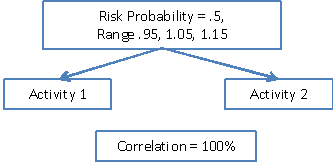
- The risk also has an impact on project activities’ durations if it does occur. This impact is specified as a range of possible impacts, stated in multiples of the activity’s estimated duration and cost – for instance low .95, most likely 1.05 and high of 1.25. These three points define a probability of impact multiplicative impact factors If the risk occurs on some iteration, the durations and costs of the activities in the schedule that the risk is assigned to will be multiplied by the same impact factor that is chosen from the impact range for that iteration.
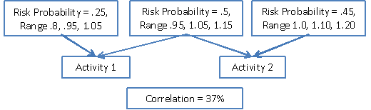
- The risks are then assigned to the activities and resources they affect. A risk can be assigned to multiple activities and an activity can be influenced by multiple risks.
The degree of correlation between the activity durations has long been understood as being important for estimating correctly project schedule risk analysis. The activity durations are uncertain, and the degree to which the impacted durations are longer and shorter together is called correlation. Correlation arises if one risk affects at least two activities’ durations. The activity durations are uncertain, and the degree to which the impacted durations are longer and shorter together is called correlation. If a risk occurs it occurs for all activities it is assigned to, and if it takes a multiplicative factor of, say, 1.12 for that iteration it is 1.12 for all of those activities. Hence, if one and only one risk affects two activities they become 100% correlated.
If, however, there are other risks that affect one activity but not the other, the correlation between the two is reduced.
The Risk Driver Method models how correlation between activity durations arises so we no longer have to estimate (guess) at the correlation coefficient between each pair of activities.
Simulation Using the Risk Driver Method
The risks’ impacts are specified as ranges of multiplicative factors that are then applied to the duration or cost of the activities to which the risk is assigned. The risks operate on the cost and schedule as follows:
- A risk has a probability of occurring on the project. If that probability is 100% then the risk occurs in every iteration. If the probability is less than 100% it will occur in that percentage of iterations.
- The risks’ impacts are specified by 3-point estimates of multiplicative factors, so a schedule risk will multiply the scheduled duration of the activity that to which it is assigned. The 3-point estimate, for instance of low 90%, most likely 105% and high 120%, is converted to a triangular distribution. For any iteration the software selects an impact multiplicative factor at random from the distribution. If the risk occurs during that iteration the multiplicative factor selected multiplies the duration of all the activities to which the risk is assigned.
Risks Applied to a Simple Case Study Schedule – Exploratory Space Probe
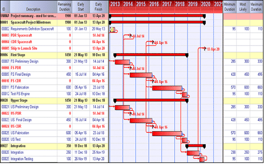
We have created a simple construction case study to illustrate the risk factors and how they are assigned to the schedule. The project is to construct a new space craft capable of sending instruments to Europa, one of Jupiter’s moons, to look for evidence of life.
We can combine the traditional 3-point estimate with Risk Drivers but we have to be careful what those estimates mean. The 3-point estimate applied directly on activity durations represents only the impact of some risk(s) on the duration and has no clear concept of the probability of a risks’ occurring. The 3-point estimates may be a good way to represent duration estimating error, which has a 100% probability of occurring but an uncertain impact. In the schedule shown below there are ranges of 95%, 100% and 110% representing an estimate judged to be from -5% to +10% of the estimate itself for each activity. These ranges are shown in the right-hand three columns in the figure.
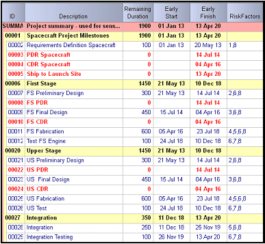
We use 7 risks that are common in real space vehicle development projects. We can add discrete risk drivers shown below, with their probability and impact parameters:
| Risk | Min | Most Likely | Max | Likelihood |
|---|---|---|---|---|
| Requirements have not been decided | 95% | 105% | 120% | 30% |
| Several alternative designs considered | 95% | 100% | 115% | 60% |
| New designs not yet proven | 90% | 103% | 112% | 40% |
| Fabrication requires new materials | 95% | 105% | 115% | 50% |
| Lost know-how since last full spacecraft | 100% | 100% | 105% | 30% |
| Funding from Congress is problematic | 90% | 105% | 115% | 70% |
| Schedule for testing is aggressive | 100% | 120%> | 130% | 100% |
These risks are then applied to the activities, as shown in the column Risk Factors below:
We are ready to simulate the schedule with estimating error and discrete risks.
Results from a Schedule Risk Simulation
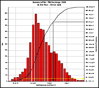
The schedule risk results from a Monte Carlo simulation are shown in the histogram for below. For a simple case study, it shows that the deterministic date of 13 April 2020 is less than 1% likely to be achieved following the current plan and without further risk mitigation actions. It is 80% likely that the current project plan with all of its risks will finish on or earlier than 7 APR 2021 or about 11.8 months later implying the need for that amount of contingency reserve of time.
Prioritizing the Risks to the Schedule
Prioritizing the risks to the schedule is one of the main benefits of the Risk Driver Method. Since we have driven the overall schedule risk with the specific project risks we can prioritize the risks for further mitigation. A listing of the risks in the case study in priority order is shown below. It is the tool that the project manager can use to improve the project’s likelihood of finishing earlier, although it is not likely that the project team can develop ways to completely mitigate all, or even any, specific risk.
The Risk Driver tornado may give a clue as to the most important risks, but it is based on correlation between variation of the risk and of the finish date, so does not represent the importance of each risk at the determined certainty target value of 80%.
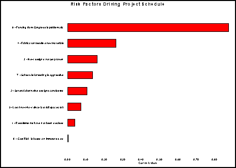
This tornado shows that “Funding from Congress is problematic” is the most important risk, probably because it is assigned to nearly all of the activities. We test that hypothesis by deleting each risk from the list (setting its probability to zero) and re-simulating for a new P-80 date. Once the most important risk is identified, we leave it out and find the next most important risk, testing several with simulations excluding the most important risk. This procedure is needed because removing the most important risk may expose paths that were not risk-critical when all risks were included. A listing of the risks in priority order is shown below. The duration estimating uncertainty is taken out last because it is different from the discrete risks and hard to mitigate except with time and gathering information:
| Explain the Contingency to the P-80 | |||
|---|---|---|---|
| P-80 Date | Take Risks Out: | ||
| All Risks In | 7-Apr-21 | Days Saved | % of Contingency |
| Specific Risks Taken Out in Order | |||
| Funding from Congress | 23-Nov-20 | 135 | 38% |
| Testing Schedule | 5-Oct-20 | 49 | 14% |
| New Materials | 3-Sep-20 | 32 | 9% |
| Alternative Design | 21-Aug-20 | 13 | 4% |
| Requirements | 14-Aug-20 | 7 | 2% |
| New Design | 6-Aug-20 | 8 | 2% |
| Lost Know How | 31-Jul-20 | 6 | 2% |
| Uncertainty | |||
| Duration Estimating | 13-Apr-20 | 109 | 30% |
| Total Contingency | 359 | 100% | |
The risk mitigation exercise starts with these priority risks. While it is unlikely to be able to fully mitigate any of these risks, the most important risks are highlighted by this table for close attention. It will be difficult if not impossible to completely mitigate a risk, so the application of resources or attention may reduce the probability of the risk from its initial estimate to a lower estimate, and may have the effect of narrowing the impact range. The benefit of the Risk Driver method is that we can decide on mitigation actions, price them and estimate the improvement in probability (lower) and impact range (narrower). Suppose the mitigation by mounting an “educational campaign” with Congress lowers the probability from 70% to 30% for this risk, but if it occurs the impact range will remain the same. In the table below we see that the P-80 is shown to be 5 January 2021 or 92 days earlier, probably justifying the investment.
| Effect of Partially Mitigating the Risk with the Highest Priority | |||||
|---|---|---|---|---|---|
| Min | Most Likely | Max | Likelihood | P-80 Date | |
| Funding from Congress is problematic | 90% | 105% | 115% | 70% | 7-Apr-21 |
Mitigation: Mount an "educational campaign" to convince Congress of the scientific and Congressional district employment benefits to funding this project. |
|||||
| Impact on the parameters | 90% | 105% | 115% | 30% | 5-Jan-21 |