Use Decision Trees to Make Important Project Decisions¹

Introduction

A large part of the risk management process involves looking into the future, trying to understand what might happen and whether it matters. An important quantitative technique which has been neglected in recent years is enjoying something of a revival – decision trees. Decision tree analysis is included in the PMBOK® Guide as one of the techniques of Quantitative Risk Analysis.

At heart the decision tree technique for making decisions in the presence of uncertainty is really quite simple, and can be applied to many different uncertain situations. For instance: Should we use the low-price bidder? Should we adopt a state-of-the-art technology?  While making many decisions is difficult, the particular difficulty of making these decisions is that the results of choosing the alternatives available may be variable, ambiguous, unknown or unknowable.

While it may be easy to make a decision for which the results are known, we need a rule to make decisions in an uncertain world. That rule is based on probability, the language most useful for describing and analyzing the future. If the future were certain we would probably decide to take the path that promises the highest value or lowest cost. With uncertainty, we will generally take the path which has the highest expected monetary value or lowest expected cost. These concepts combine the probability that an event will occur with the impact if it does; in other words, expected monetary value and expected cost follow the definition of project risk in the PMBOK® Guide (namely “an uncertain event or condition that, if it occurs, has a positive or negative effect on at least one project objective”).

Many decisions are like this in risky projects, and we often need to make a decision even if we do not know for sure how it will turn out. These can be very important decisions for the project, and making them correctly increases the possibility of project success.

Simple Decision –
One Decision Node and Two Chance Nodes

We can illustrate decision tree analysis by considering a common decision faced on a project. We are the prime contractor and there is a penalty in our contract with the main client for every day we deliver late. We need to decide which sub-contractor to use for a critical activity. Our aim is to minimize our expected cost. It is often difficult to argue for using the higher-priced sub-contractor, even if that one is known to be reliable. The lower-bidding sub-contractor also promises a successful delivery, although we suspect that he cannot do so reliably.  A rigorous analysis of this decision using a simplified decision tree structure that minimizes our expected cost is shown below:

• One sub-contractor is lower-cost ($110,000 bid). We estimate however that there is a 50% chance that this contractor will be 90 days late and our contract with the main client specifies that we must pay a delay penalty of $1,000 per calendar day for every day we deliver late.


• The higher-cost sub-contractor bids $140,000. We know this contractor and assess that it poses a low 10% chance of being late, and only 30 days late at that. Of course, our customer will impose on us the same $1,000 delay penalty per day for late delivery.

We need to know if there is any benefit to using the higher-cost sub-contractor, and we suspect it may lie in the greater reliability of performance we expect.  Of course, both we and our customer need to be convinced of the benefit.  A formal analysis using decision trees will ascertain if there is a benefit, and will also document it for the customer.

The steps we need to implement are as follows:

• Identify the major decisions to be made (decision nodes) and the major uncertainties (event nodes) that relate to the consequences.


• Construct the structure of the decision and all of its (main) consequences. Because each decision or event node has at least two alternatives, the structure of the decision looks like a tree, typically placed on its side with the root on the left and the branches on the right, with potentially many branches.

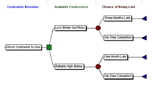
• Estimate the costs and benefits of each alternative decision. This is usually a task of some importance since the final result of the decision tree analysis will depend largely on the accuracy of these comparative estimates.


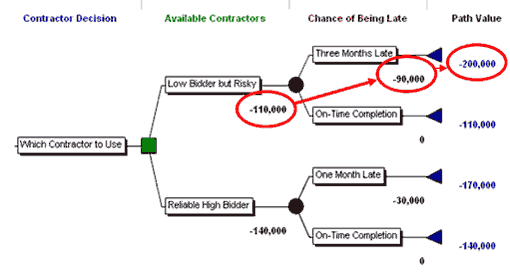
• Calculate the value of the project for each path, beginning on the left-hand side with the first decision and cumulating the values to the final branch tip on the right as if each of the decisions were taken and each event occurred. This action is called “rolling forward.” For example, taking the top-most branch, the lower bidder bids $110,000 and if we are 90 days late because he is late, $90,000 in penalties will be added by our customer for a total cost to us of $200,000. This rolling forward calculation of the four possible path values is shown in Figure 2 below.

• To identify the correct decision and its value (to “solve the tree”) we need to estimate some additional data, namely the probability of each possible uncertain outcome. Estimating these probabilities is not as easy as it might appear, since there are often no useful databases from which to extract the data.  Expert judgment is usually required and that judgment may be poorly-informed or biased.


• To solve the tree we must calculate the value of each node – including both chance nodes and decision nodes. We start with the path values at the far right-hand end of the tree and then moving from the right to the left calculate the value of each node as it is encountered.  This process is called “folding back” the tree.
  
  

  The rules for finding the values of the chance and decision nodes are:

  • The value of each chance node is found by multiplying the values of the uncertain alternatives by their probabilities of occurring and sum the results. This value is known as Expected Monetary Value (EMV).
  
  
  • The value of a decision node is the highest value of the succeeding branches leading from that node.

  This procedure is illustrated in Figure 3 below.

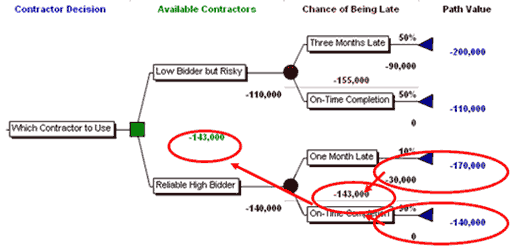
The “folding back” calculations for our simple example are as follows:

• For the “Low Bidder but Risky” alternative
  1. Multiply -$200,000 by 50% for -$100,000
  2. Multiply -$110,000 by 50% for -$55,000
  3. Add these numbers (- $100,000 - $55,000) for - $155,000. This is the Expected Cost of this option, since it is 50% likely that the low bidder will be late.
  
  
• For the Reliable High Bidder
  1. Multiply -$170,000 x 10% for - $17,000
  2. Multiply  -$140,000 x 90% = - $126,000
  3. Add the results (- $17,000 and - $126,000) for - $143,000

In the Contractor Decision case there is only one decision node, the original one. The alternatives are:

1. Low Bidder but Risky at -$155,000
2. Reliable High Bidder at -$143,000.

Clearly, the reliable high bidder has the edge here and is actually expected to cost less for the project because of their greater on-time reliability. The value of the process is to represent the values corrected for, or incorporating in, their uncertainty.

Tree with Embedded Decision Nodes – The Value of “Folding Back”

For simple decision trees with just one decision and chance nodes like the one in our earlier example, the full value of the folding back technique is not evident. However, many decision trees on real projects contain embedded decision nodes. The only way to solve such decision trees is to use the folding back technique from right to left. This is because the value of each node depends on the values of those nodes to its right (in the standard left-to-right orientation of decision trees depicted here).

In folding back, the right-hand-most nodes must be valued before those next in right-to-left order, as shown in the following example using a technology decision.

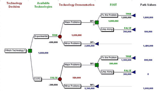
In this decision tree, we are faced with the choice of using an experimental technology or a commercial-off-the-shelf (COTS) technology. If it is successful, the experimental technology promises greater rewards.  Of course both solutions could encounter “Minor Problems”, which we are prepared to accept. But unfortunately, we need to acknowledge that both alternative solutions carry a possibility of “Major Problems”. This is quite likely with the Experimental technology for which we estimate an 80% probability of such problems, but even COTS have a 10% chance of major problems. If major problems occur, we must decide whether to fix the problem or to “limp along.” Because of this decision there is an embedded decision node in each branch after a chance node in this more realistic decision tree.

The folding back process starts at the right-hand-side of the tree, at the end of the branches. On each branch we encounter a decision node first. We have estimated rewards to the “Limp Along” scenario and the “Fix the Problem” scenario. Each of these is probably a net present value (NPV) of future income streams with the latter, Fix the Problem, netting out the cost of the actions necessary to perform the fix. 

With both the Experimental and COTS technologies, the decision would be to FIX the Problem if major problems occur since to “Limp Along” provides small rewards. The value (not the “Expected Monetary Value” at this point since it is a decision rather than a chance node) of the decision node is found by folding back from the right toward the left using the path values. That value is found by selecting the highest path value offered:

1. $800,000 in the case of the COTS decision
2. $1,000,000 for the experimental technology.

There is no other way to discover this value than starting from the right-hand side of the tree and folding back.

The values of the embedded decision nodes, $1,000,000 and $800,000, are then carried to the left and used in the Expected Monetary Value (EMV) calculations that provide the value of the two event nodes.  The calculations are as follows for the COTS branch:

1. Multiply the value of the “major problems” node by its probability ($800,000 x 10%) for the value $80,000.


2. We multiply the path value of the “minor problems by its probability ($1,000,000 x 90%) for a value of $900,000.


3. Add the two values together for $980,000. This is the EMV of the COTS decision

To find the value of using the experimental technology:

1. Multiply the value of the major problems branch by its probability ($1,000,000 x 80%) for a total of $800,000


2. Multiply the path value of the minor problems branch by its probability ($1,400,000 x 20%) for the total of $280,000.


3. Add these two values together to derive the EMV of the branch, $1,080,000.

The ultimate decision in the technology case is found by comparing the EMVs of two technologies. This comparison indicates that we should choose the experimental technology because, even though there is an 80% probability of major problems, the technology’s EMV is higher than that for the COTS choice. The closeness of these values, $1,080,000 vs. $980,000, indicates that this decision is close. The decision is quite sensitive to the accuracy of the estimates and we are encouraged to both (1) make these estimates as accurate as possible, and (2) evaluate factors that are not included in the decision tree, for instance whether proving the experimental technology on this project might lead to future licensing revenues, which may affect our decision.

The Risk Averse Organization

In the examples above we have assumed that the organization wants to choose whichever decision maximizes its expected monetary value or minimizes its expected cost.  This behavior, which could be called “risk-neutral,” may represent an organization that has many projects and can thrive if it succeeds “on the average.” 

Many, if not most, organizations are cautious in situations where they think they might be vulnerable to large losses. These organizations may shy away from project decisions which, if they were to fail, would expose the organization to the probability of large losses, even if such project decisions might also offer a possibility of large gains associated with success.  This behavior might be called “risk-averse”.  Decisions made by risk-averse organizations’ tend to maximize their expected utility rather than expected value, and that utility may give serious (negative) weight to the possibility of large losses.  Most decision tree software allows the user to design a utility function that reflects the organization’s degree of aversion to large losses.

Conclusion

Project decisions, even quite simple ones, can be difficult to make because their implications are often not certain.  This is a fact of life for most project managers, who often face situations like those explored above: the choice of alternative contractors and of alternative technologies. Each of these decisions poses clear alternatives but murky consequences. Uncertain consequences are best described and analyzed using probability concepts as part of a decision tree analysis to maximize Expected Monetary Value or minimize expected costs to the organization.

Decision trees allow project managers to distinguish between decisions where we have control and chance events that may or may not happen. It takes account of the costs and rewards of decision options as well as the probabilities and impacts of associated risks. Structured analysis using “rolling forward” and “folding back” allows the best decision option to be taken based on calculation of Expected Monetary Value, although this may be influenced by the risk appetite of the organization. The decision tree technique offers a powerful way of describing, understanding and analyzing uncertainty, and can be a valuable part of the toolkit for any project manager who needs to make decisions where the outcome is uncertain.